OLAP with Apache Phoenix and HBase
Today's blog is brought to you by Juan Rodríguez Hortalá of LAMBDOOP
One of the benefits of having a SQL query interface for a database is that SQL has become a lingua franca that is used as the basis for the interoperability of many systems. One example of that are visualization tools, that usually accept SQL connections as data sources. In this post we'll see how to use Apache Phoenix as a bridge between HBase and Saiku Analytics, a visualization tool for Business Intelligence.
Saiku is an open source visualization tool for Online Analytical Processing (OLAP) that consists in modeling a given business process as a set of facts corresponding to business transactions, that contain measures of quantities relevant for the business, and which are categorized by several dimensions that describe the context of the transaction.
For example if we want to analyze the traffic of a website then we might define a measure ACTIVE_VISITOR for the number of visitors and put it into context by considering the date of the visit (DATE dimension), or the part of the site which was visited (FEATURE dimension).
Facts and dimensions are collected into a logical (and sometimes also physical) structure called OLAP cube, which can be thought as a multidimensional array indexed by the dimensions and with the measures as values. OLAP cubes are queried using MultiDimensional eXpressions (MDX), a query language for specifying selections and aggregations in a natural way over the multidimensional structure of a cube. And here comes Saiku! Saiku is an OLAP front-end for visualizing the results of MDX queries, both in tabular format or as different types of charts, and that also offers a drag and drop interface for generating MDX queries.
Saiku accepts several data sources, and in particular it is able to use the Mondrian server to implement ROLAP, which is a popular technique for OLAP that uses a relational database to store and compute the cubes. Did I say relational? Well, in fact all that Mondrian needs is a JDBC driver ... And this leads us to this post, where I'll share my experiences combining Phoenix with Mondrian to use HBase as the analytical database in the backend of an OLAP system with Saiku as the front-end. As there are a few layers in this setting, let's describe the flow of a query in this system before entering into more details:
-
Saiku uses an schema file provided during configuration that contains the declarations of some OLAP cubes, and displays the dimensions and measures of the cubes to the user.
-
The user selects a cube and builds a query using Saiku’s drag and drop interface over the cube.
-
Saiku generates an MDX expression and passes it to Mondrian for execution.
-
Mondrian compiles the MDX expression into an SQL query, and then uses Phoenix JDBC to execute it.
-
HBase executes the query and then gives the results back to Phoenix.
-
Phoenix passes the results to Mondrian, which passes them to Saiku, which then renders the results as a table in the user interface.
Setup and example
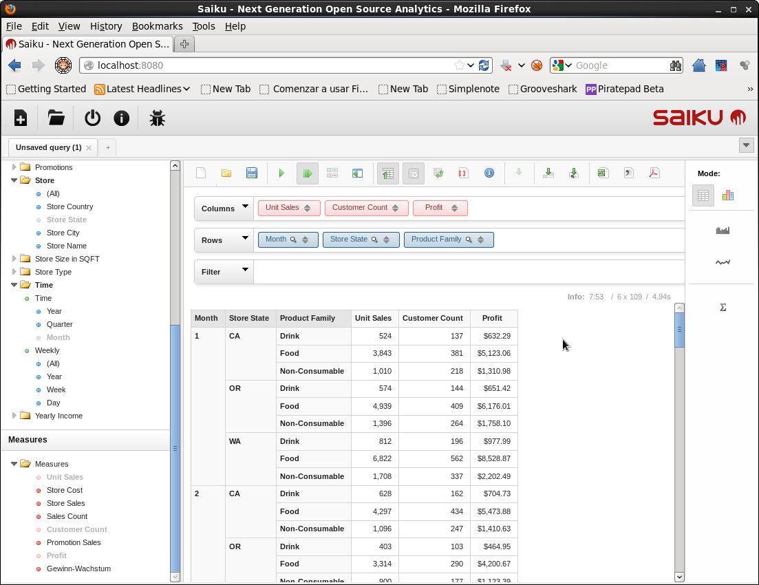
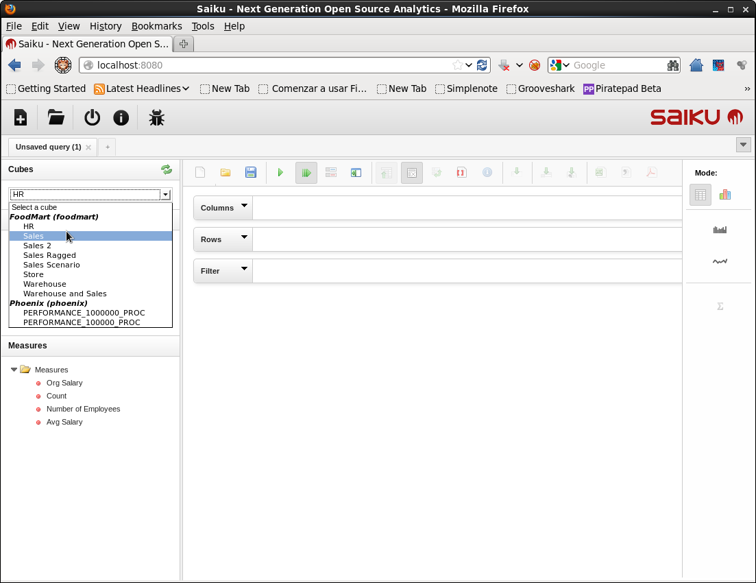
We’ll see how to setup Saiku to work with Phoenix with a simple example. This procedure has been tested in a Cloudera Quickstart VM for CDH 4.4.0, which is shipped with HBase 0.94.6, therefore we’ll be using Phoenix 3. First of all we have to download phoenix 3 and install it by copying phoenix-core-*.jar in the classpath of each region server (for example at /usr/lib/hbase/lib/) and then restarting them. Regarding Saiku, it can be installed as a Pentaho BA Server plugin, or as a stand alone application as we'll do in this tutorial. To do that just download Saiku Server 2.5 (including Foodmart DB) and extract the compressed file, which contains a Tomcat distribution with Saiku installed as a webapp. To start and stop Saiku use the scripts start-saiku.sh and stop-saiku.sh. By default Saiku runs at port 8080 and uses ‘admin’ as both user and password for the login page. After login you should see be able to select one of the cubes of the Foodmart DB at the combo at the upper left corner of the UI.
Now it’s time to connect Saiku to Phoenix. The first step is defining the structure of the OLAP cube we are going to analyze. In the example above we considered analyzing the traffic of a website by measuring quantities like the number of visitors along dimensions like the date of the visit or the part of the site that was visited. This happens to correspond to the structure of the PERFORMANCE tables created by the script bin/performance.py shipped with Phoenix. So let’s run the command bin/performance.py localhost 100000 so a table PERFORMANCE_100000 with 100.000 rows with the following schema is created:
CREATE TABLE IF NOT EXISTS PERFORMANCE_100000 (
HOST CHAR(2) NOT NULL, DOMAIN VARCHAR NOT NULL,
FEATURE VARCHAR NOT NULL, DATE DATE NOT NULL,
USAGE.CORE BIGINT, USAGE.DB BIGINT, STATS.ACTIVE_VISITOR INTEGER
CONSTRAINT PK PRIMARY KEY (HOST, DOMAIN, FEATURE, DATE)
) SPLIT ON ('CSGoogle','CSSalesforce','EUApple','EUGoogle',
'EUSalesforce', 'NAApple','NAGoogle','NASalesforce');
In this table the 4 columns that compose the primary key correspond to the dimensions of the cube, while the other 3 columns are the quantities to be measured. That is a fact table with with 4 degenerate dimensions (see e.g. Star Schema The Complete Reference for more details about dimensional modeling), that represents and OLAP cube. Nevertheless there is a problem with this cube: the granularity for the time dimension it’s too fine, as we can see in the following query.
0: jdbc:phoenix:localhost> SELECT TO_CHAR(DATE) FROM PERFORMANCE_1000000 LIMIT 5;
+---------------+
| TO_CHAR(DATE) |
+---------------+
| 2014-05-15 09:47:42 |
| 2014-05-15 09:47:50 |
| 2014-05-15 09:49:09 |
| 2014-05-15 09:49:23 |
| 2014-05-15 09:49:44 |
+---------------+
5 rows selected (0.161 seconds)
We have a resolution of seconds in the DATE column, so if we grouped values by date we would end up with a group per record, hence this dimensions is useless. To fix this we just have to add a new column with a coarser granularity, for example of days. To do that we can use the following script, that should be invoked as bash proc_performance_table.sh
#!/bin/bash
if [ $# -ne 2 ]
then
echo "Usage: $0
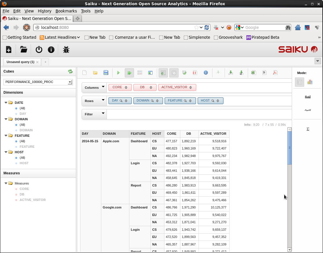
exit 1 fi PHOENIX_BIN_DIR=$1 IN_TABLE=$2 OUT_TABLE="${IN_TABLE}_PROC" echo "Table $OUT_TABLE will be created" pushd $PHOENIX_BIN_DIR ./sqlline.py localhost < CREATE TABLE IF NOT EXISTS $OUT_TABLE ( HOST CHAR(2) NOT NULL, DOMAIN VARCHAR NOT NULL, FEATURE VARCHAR NOT NULL, DATE DATE NOT NULL, DATE_DAY DATE NOT NULL, USAGE.CORE BIGINT, USAGE.DB BIGINT, STATS.ACTIVE_VISITOR INTEGER CONSTRAINT PK PRIMARY KEY (HOST, DOMAIN, FEATURE, DATE)) SPLIT ON ('CSGoogle','CSSalesforce','EUApple','EUGoogle','EUSalesforce', 'NAApple','NAGoogle','NASalesforce'); !autocommit on UPSERT INTO $OUT_TABLE SELECT HOST, DOMAIN, FEATURE, DATE, TRUNC(DATE, 'DAY') as DATE_DAY, USAGE.CORE, USAGE.DB, STATS.ACTIVE_VISITOR FROM $IN_TABLE; !quit END echo "Done" popd That creates a new table PERFORMANCE_100000_PROC with an extra column DATE_DAY for the date with a resolution of days. We’ll perform the analysis over this table. The next step is creating a Mondrian schema that maps an OLAP cube to this table, for Mondrian to know which column to use as a dimension, and how to define the measures. Create a file Phoenix.xml with the following contents:
There we have declared an schema “Phoenix” containing a single cube “PERFORMANCE_100000_PROC” defined over the table “PERFORMANCE_100000_PROC”. This cube has 4 dimensions with a single level, that corresponds to the columns HOST, DOMAIN, FEATURE and DATE_DAY, and 3 metrics that are computed adding the values in the groups determined by the dimensions, over the columns CORE, DB and ACTIVE_VISITOR. As we can see in tomcat/webapps/saiku/WEB-INF/lib/mondrian-3.5.7.jar, this version of Saiku (2.5) uses Mondrian 3, so take a look at the Mondrian 3 documentation or to Mondrian in Action for more information about Mondrian schemas if you are interested. Now we have to create a new Saiku data source that uses this schema, by creating a file type=OLAP name=phoenix driver=mondrian.olap4j.MondrianOlap4jDriver location=jdbc:mondrian:Jdbc=jdbc:phoenix:localhost;Catalog=res:phoenix/Phoenix.xml;JdbcDrivers=org.apache.phoenix.jdbc.PhoenixDriver That declares an OLAP connection named phoenix that uses Mondrian as the driver, and Phoenix as JDBC. We just need to do a couple more things for this to work: Add the jars for Phoenix, HBase and Hadoop to Saiku’s classpath, by copying phoenix-*client-without-hbase.jar, /usr/lib/hbase/hbase.jar, /usr/lib/hadoop/hadoop-common.jar and /usr/lib/hadoop/hadoop-auth.jar into Create a directory Now restart Saiku and the new cube should appear. I suggest watching tomcat/logs/catalina.out and tomcat/logs/saiku.log at the Saiku install path for possible errors and other information. If we take a look to saiku.log we can see the MDX query generated by Saiku, and the running time for the query in HBase. These execution times are for a Cloudera Quickstart VM running on VMware Player with 4448 MB RAM and 4 cores, in a laptop with an i7 processor and 8 GB RAM, and with default settings for HBase, Phoenix and Saiku. 2014-05-18 09:20:58,225 DEBUG [org.saiku.web.rest.resources.QueryResource] TRACK /query/CC92DB19-D97E-E68D-B927-E6259DB6BF70/resultflattened GET 2014-05-18 09:20:58,226 INFO [org.saiku.service.olap.OlapQueryService] runId:2 Type:QM: SELECT NON EMPTY {[Measures].[CORE], [Measures].[DB], [Measures].[ACTIVE_VISITOR]} ON COLUMNS, NON EMPTY CrossJoin([DATE].[DAY].Members, CrossJoin([DOMAIN].[DOMAIN].Members, CrossJoin([FEATURE].[FEATURE].Members, [HOST].[HOST].Members))) ON ROWS FROM [PERFORMANCE_100000_PROC] 2014-05-18 09:20:59,220 INFO [org.saiku.service.olap.OlapQueryService] runId:2 Size: 7/55 Execute: 970ms Format: 24ms Total: 994ms The same query for a performance table of 1 million records is completed in an order of 8 to 18 seconds in the same setting. That's all! The next natural step would be defining a richer star schema with independent dimension tables, and testing the limits of Phoenix's star-join optimization. I hope this post has encouraged you to try it yourself. "